Cinestyle: matplotlib themes pulled from film

Cinestyle is a Python package I wrote to give matplotlib a handful of opinionated styles — Film Noir, Studio Ghibli, Wes Anderson, Blade Runner, Star Wars. Each is a thin wrapper around rcParams and a few helper methods. Nothing exotic. The point was a chart that looks like the thing instead of the default.

The examples below run on 50,000 IMDB reviews — 25,000 positive, 25,000 negative. Code, repo, and the five resulting figures follow.

Source: github.com/Burton-David/cinematic-matplotlib

The data

50,000 IMDB reviews, evenly split between positive and negative. Mean review length is 1,309 characters (231 words). The vocabulary asymmetry is small but real: negative reviewers say movie more often (34,811 vs. 26,681), positive reviewers say film more often (29,367 vs. 25,719).

Five styles

1. Film Noir — sentiment distribution

High contrast, deep blacks, a single bold red. Useful when the chart needs to read as a comparison and nothing else.

import pandas as pd
import matplotlib.pyplot as plt
from cinestyle import FilmNoir

# Load data
df = pd.read_csv('IMDB Dataset.csv')

# Initialize Film Noir style
noir = FilmNoir()
fig, ax = plt.subplots(figsize=(12, 8))
noir.style_axes(ax)

# Create bar chart
sentiments = df['sentiment'].value_counts()
bars = ax.bar(sentiments.index, sentiments.values,
              color=['#8B0000', '#FFFFFF'],
              edgecolor='white', linewidth=2, width=0.6)

ax.set_title("LIGHT VS DARK: SENTIMENT DISTRIBUTION",
             color='white', fontsize=22, fontweight='bold', pad=20)
ax.set_ylabel('Review Count', color='white', fontsize=14)

# Add value labels
for bar in bars:
    height = bar.get_height()
    ax.text(bar.get_x() + bar.get_width()/2., height,
            f'{int(height):,}',
            ha='center', va='bottom', color='white',
            fontsize=16, fontweight='bold')

plt.savefig('noir_sentiment.png', dpi=300, bbox_inches='tight',
            facecolor='#121212')
plt.show()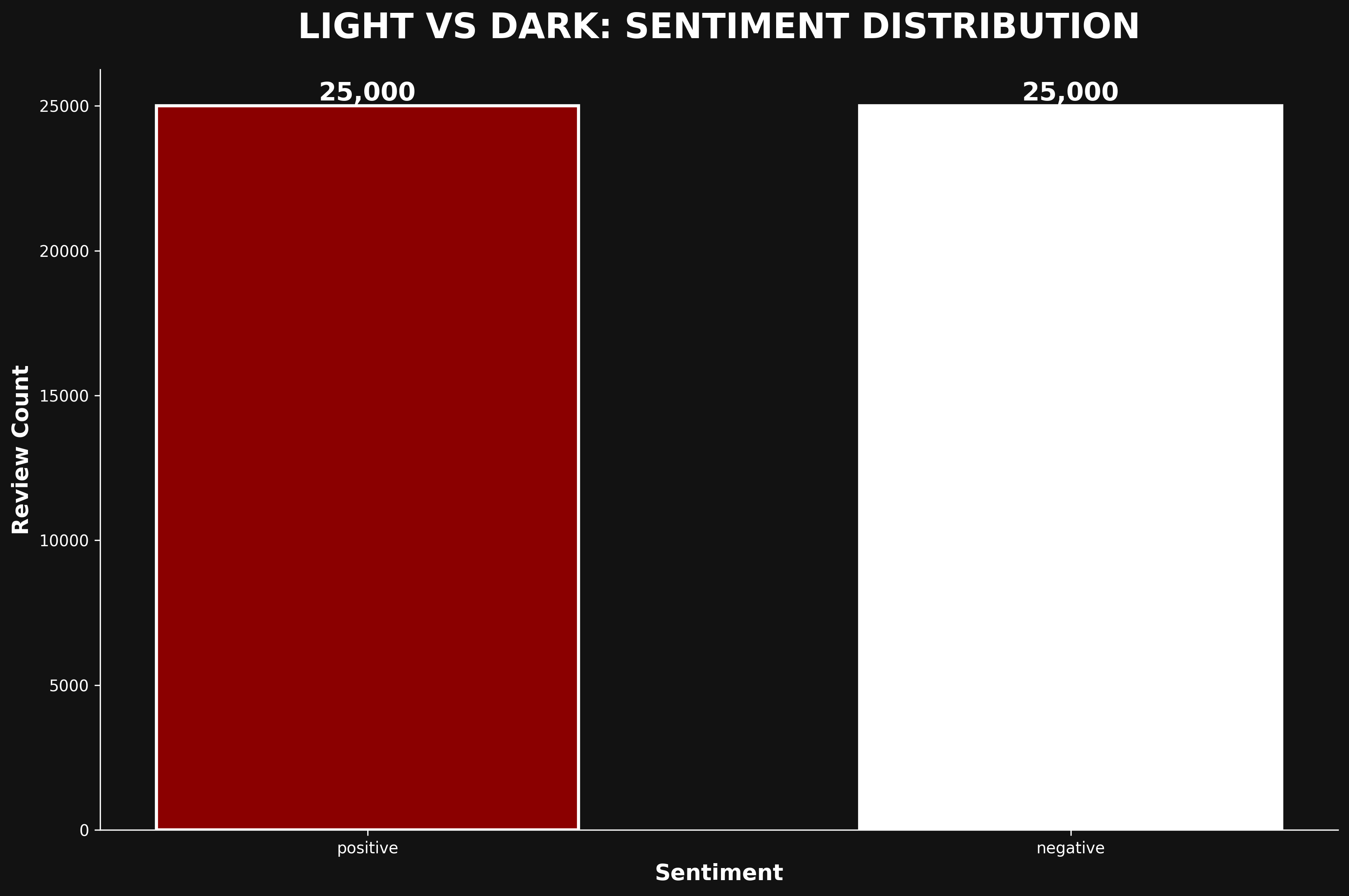

Best for: binary comparisons. Two categories, sharp difference, nothing else competing for attention.

---

2. Studio Ghibli — review length distribution

Soft greens, pastoral palette, organic edges. Distributions read as continuous rather than categorical.

from cinestyle import Ghibli

# Calculate review lengths
df['review_length'] = df['review'].str.len()

# Initialize Ghibli style
ghibli = Ghibli()
fig, ax = plt.subplots(figsize=(14, 8))
ghibli.style_axes(ax)

# Create histogram
ax.hist(df['review_length'], bins=60, color='#90EE90',
        alpha=0.7, edgecolor='#2F4F2F', linewidth=1.5)

ax.set_title("The Flow of Words: Review Length Distribution",
             fontsize=20, pad=20, fontweight='600')
ax.set_xlabel('Character Count', fontsize=14)
ax.set_ylabel('Number of Reviews', fontsize=14)

# Add mean line
mean_length = df['review_length'].mean()
ax.axvline(mean_length, color='#8B4513', linestyle='--',
           linewidth=2.5, label=f'Mean: {mean_length:.0f} characters')
ax.legend(fontsize=12)

plt.savefig('ghibli_length.png', dpi=300, bbox_inches='tight')
plt.show()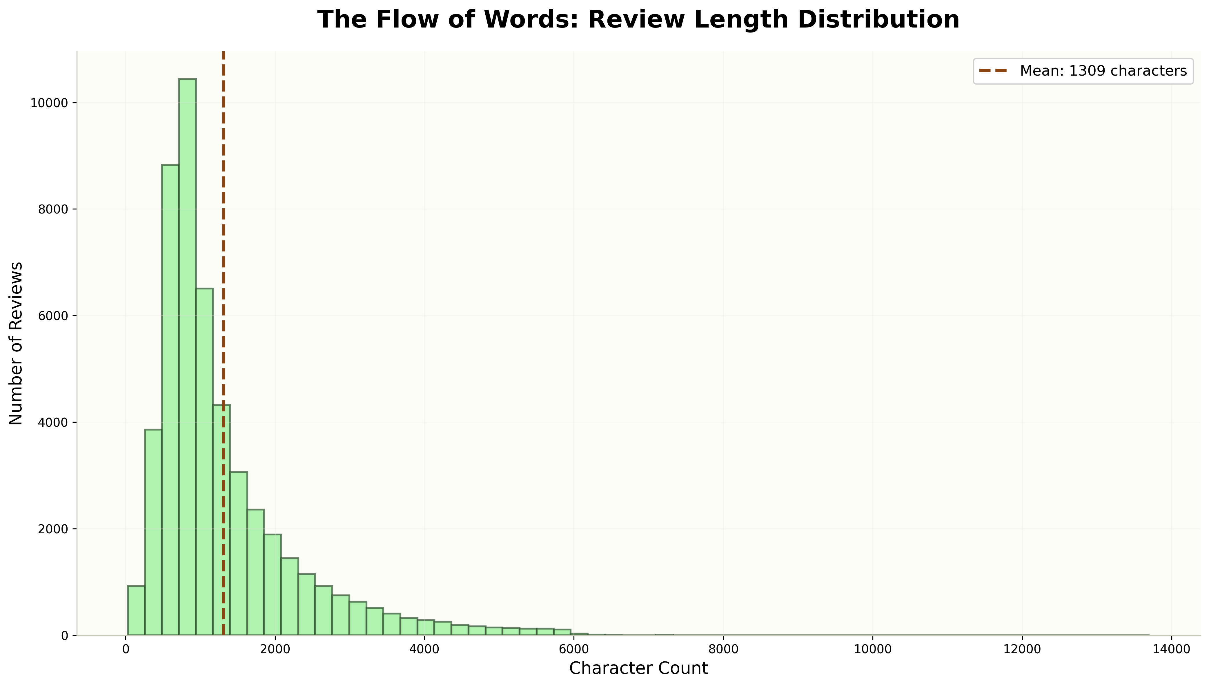

Median review length is 970 characters; the distribution stretches from 32 to 13,704.

Best for: histograms and distributions. Anything where you want the eye to follow shape rather than count bars.

---

3. Wes Anderson — word frequency comparison

Pastels arranged symmetrically. Two panels side by side, equal weight, balanced composition.

from cinestyle import WesAnderson
from collections import Counter

# Get top words by sentiment
def get_top_words(reviews, n=10):
    words = ' '.join(reviews).lower().split()
    stopwords = {'the', 'a', 'an', 'and', 'or', 'but', 'in', 'on',
                 'at', 'to', 'for', 'of', 'is', 'it', 'this', 'that'}
    words = [w for w in words if w not in stopwords and len(w) > 3]
    return Counter(words).most_common(n)

pos_words = get_top_words(df[df['sentiment']=='positive']['review'])
neg_words = get_top_words(df[df['sentiment']=='negative']['review'])

# Initialize Wes Anderson style
wes = WesAnderson()
fig, (ax1, ax2) = plt.subplots(1, 2, figsize=(18, 8))
wes.style_axes(ax1)
wes.style_axes(ax2)

# Positive words panel
pos_labels = [w[0] for w in pos_words]
pos_values = [w[1] for w in pos_words]
ax1.barh(pos_labels, pos_values, color='#F4A460',
         edgecolor='#8B4513', linewidth=1.5)
ax1.set_title("Positive Words", fontsize=18, fontweight='600')
ax1.invert_yaxis()

# Negative words panel
neg_labels = [w[0] for w in neg_words]
neg_values = [w[1] for w in neg_words]
ax2.barh(neg_labels, neg_values, color='#9370DB',
         edgecolor='#4B0082', linewidth=1.5)
ax2.set_title("Negative Words", fontsize=18, fontweight='600')
ax2.invert_yaxis()

fig.suptitle('A Symmetrical Study of Sentiment',
             fontsize=22, fontweight='bold', y=0.98)

plt.savefig('wes_anderson_words.png', dpi=300, bbox_inches='tight')
plt.show()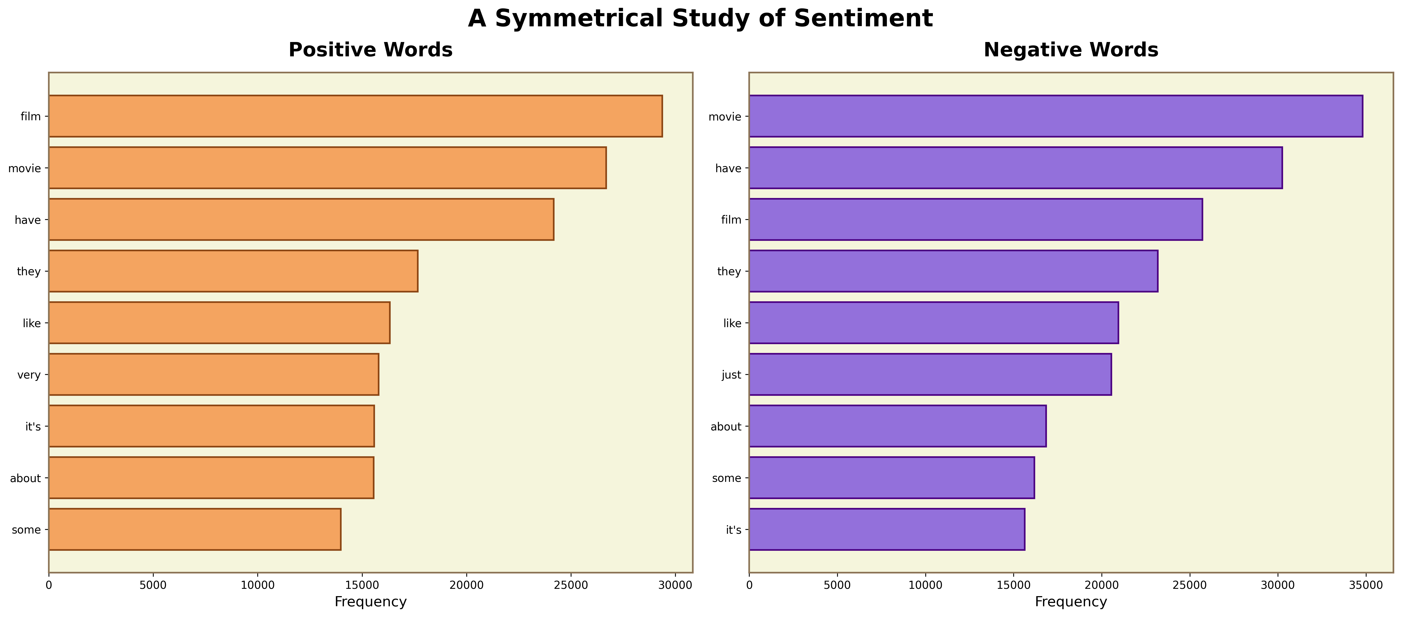

The top words overlap heavily between sentiments. Negative leans on movie (34,811) and just (20,544); positive leans on film (29,367) and very (15,791).

Best for: paired comparisons. Two populations, same axes, the symmetry does the work.

---

4. Blade Runner — word count scatter

Cyan and magenta on near-black. The cyberpunk reading is intentional but the practical point is that two semi-transparent colors over a dark field separate well at high overplotting.

from cinestyle import BladeRunner

# Calculate word counts
df['word_count'] = df['review'].str.split().str.len()

# Initialize Blade Runner style
blade = BladeRunner()
fig, ax = plt.subplots(figsize=(12, 8))
blade.style_axes(ax)

# Sample for performance
positive = df[df['sentiment']=='positive'].sample(2000, random_state=42)
negative = df[df['sentiment']=='negative'].sample(2000, random_state=42)

# Create scatter plot
ax.scatter(positive.index, positive['word_count'],
           c='#00FFFF', alpha=0.5, s=20, label='Positive')
ax.scatter(negative.index, negative['word_count'],
           c='#FF00FF', alpha=0.5, s=20, label='Negative')

ax.set_title("WORD COUNT PATTERNS", color='cyan',
             fontsize=20, fontweight='bold')
ax.set_xlabel('Review Index', color='cyan')
ax.set_ylabel('Word Count', color='cyan')
ax.legend(facecolor='#0a0a0a', edgecolor='#00FFFF')

plt.savefig('blade_runner_scatter.png', dpi=300, bbox_inches='tight',
            facecolor='#0a0a0a')
plt.show()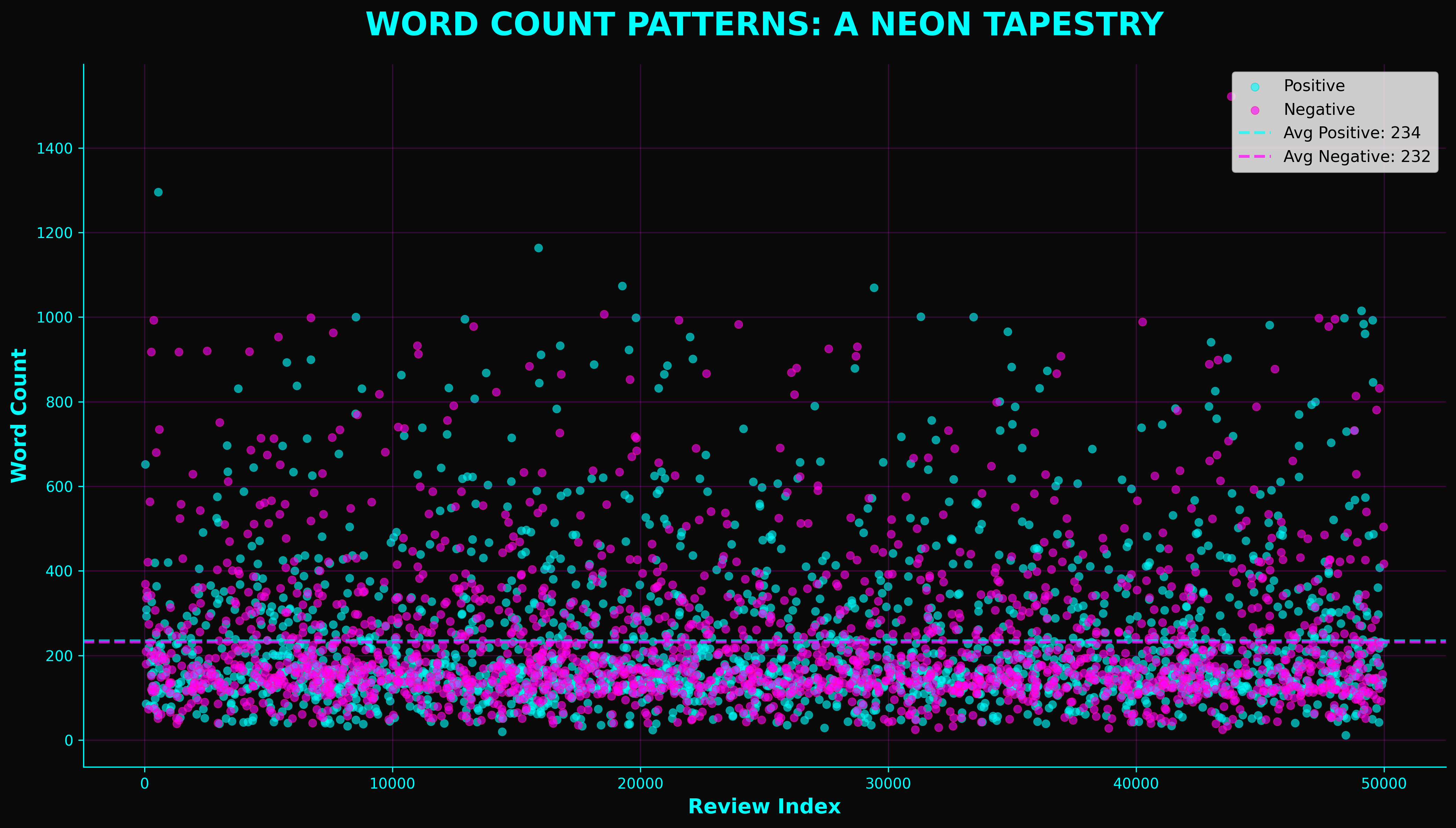

Positive reviews run 233 words on average, negative 229. Median across both is 173. The visual point is that the two sentiment classes are almost completely interpenetrating — sentiment is not encoded in length.

Best for: dense scatter plots, especially two overlapping populations.

---

5. Star Wars — keyword ranking

Gold and blue alternating on pure black. Reads as a list of things you should care about.

from cinestyle import StarWars

# Get top 20 keywords across all reviews
all_words = get_top_words(df['review'], n=20)

# Initialize Star Wars style
starwars = StarWars()
fig, ax = plt.subplots(figsize=(14, 8))
starwars.style_axes(ax)

# Create horizontal bar chart
words = [w[0] for w in all_words]
counts = [w[1] for w in all_words]
colors = ['#FFD700', '#1E90FF'] * 10

ax.barh(words, counts, color=colors, edgecolor='#FFD700', linewidth=1.5)
ax.set_title("EPIC KEYWORD UNIVERSE", color='gold',
             fontsize=22, fontweight='bold')
ax.set_xlabel('Frequency', color='gold', fontsize=14)
ax.invert_yaxis()

# Add value labels
for i, (word, count) in enumerate(all_words):
    ax.text(count, i, f'  {count:,}', va='center',
            color='gold', fontsize=11, fontweight='bold')

plt.savefig('star_wars_keywords.png', dpi=300, bbox_inches='tight',
            facecolor='black')
plt.show()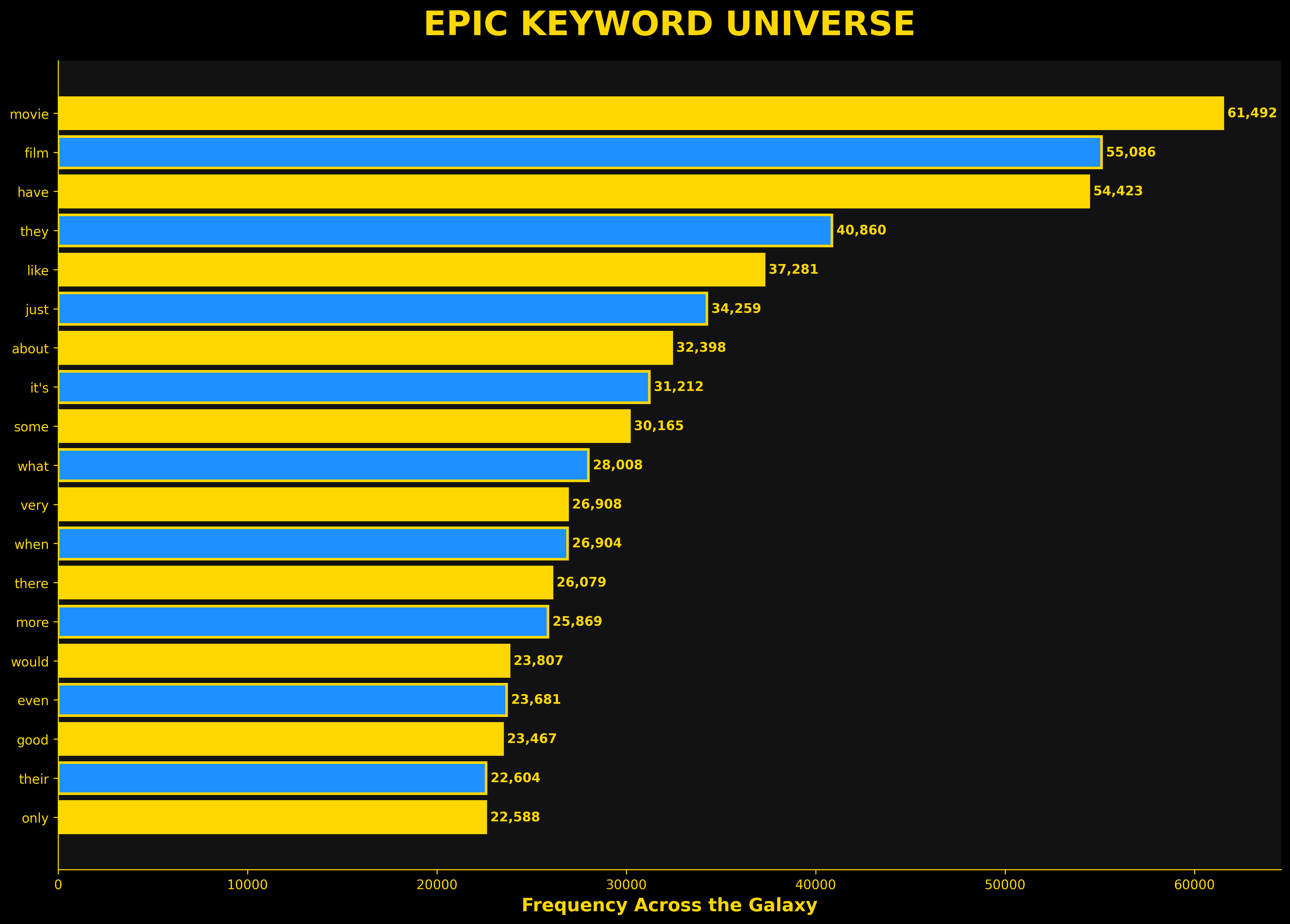

Top tokens across the whole corpus: movie (61,492), film (55,086), have (54,423), they (40,860), like (37,281).

Best for: rankings. Top-N lists, leaderboards, ordered categoricals.

---

Install and basic usage

git clone https://github.com/Burton-David/cinematic-matplotlib.git
cd cinematic-matplotlib
pip install -e .

import matplotlib.pyplot as plt
from cinestyle import FilmNoir, Ghibli, WesAnderson, BladeRunner, StarWars

noir = FilmNoir()
fig, ax = plt.subplots(figsize=(12, 8))
noir.style_axes(ax)

ax.plot([1, 2, 3], [4, 5, 6])
plt.show()

Quick reference

Style	Best for	Look
Film Noir	Binary comparisons, stark contrasts	Black, white, blood red
Studio Ghibli	Histograms, distributions	Soft greens, pastoral
Wes Anderson	Paired comparisons	Pastel, symmetrical
Blade Runner	Dense scatter, overlapping classes	Cyan/magenta on black
Star Wars	Rankings, top-N lists	Gold and blue on black

Under the hood

Each style does three things: sets rcParams (fonts, weights, backgrounds), defines a small palette, and exposes a style_axes(ax) method that applies the look to a specific axes. That’s the whole library. You can also call apply_style() to set the global rcParams once and then use matplotlib normally:

noir = FilmNoir()
fig, ax = plt.subplots()
noir.apply_style()
noir.style_axes(ax)
ax.plot(x, y, color=noir.colors['primary'])

Repo: github.com/Burton-David/cinematic-matplotlib.