Classifying Wine

Three chemical readings, alcohol, proline, and flavanoids, get you to 94.4% on a test set you never touched during training. The full 13-feature model gets 98.1%. Less than four points separates them, and that gap is all that thirteen features and their interactions buy you over three. If someone told me a gradient-boosted ensemble was needed here, I would ask them to look at the data first.

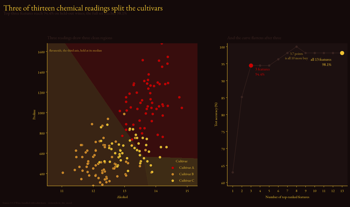
Three features carve three clean regions. The accuracy curve holds at 94.4% from three to five features, then climbs to 100% at eight, so more features do buy something, just not much. Everything below is me checking that the picture is honest.

The data is the UCI Wine set, bundled with scikit-learn: 178 bottles, 13 chemical measurements each, sorted into three cultivars. The classes are 59, 71, and 48, close enough to balanced that I did not have to think about it. Every measurement is a real lab readout: alcohol percentage, magnesium in mg/L, color intensity, the proline content that grapes accumulate differently by variety.

The simplest thing first

I split 70/30, stratified, fixed the seed, and scaled the features with a StandardScaler fit on the training rows only, so no information from the test set leaks back through the mean and variance. Then plain multinomial logistic regression. No regularization sweep, no kernel.

Test accuracy: 98.1%. On a 54-row test set that is a single misclassified bottle. So the headline result for “throw everything at it” is one mistake out of 54. It raises the obvious question: how much of that came from the thirteen features, and how much from two or three of them carrying the others?

What actually carries the signal

I ranked features by the mean absolute standardized coefficient across the three class coefficient vectors. Standardized, because the scaler lives inside the pipeline, so the coefficients are comparable across features that live on wildly different units. Proline runs into the hundreds; hue sits below two.

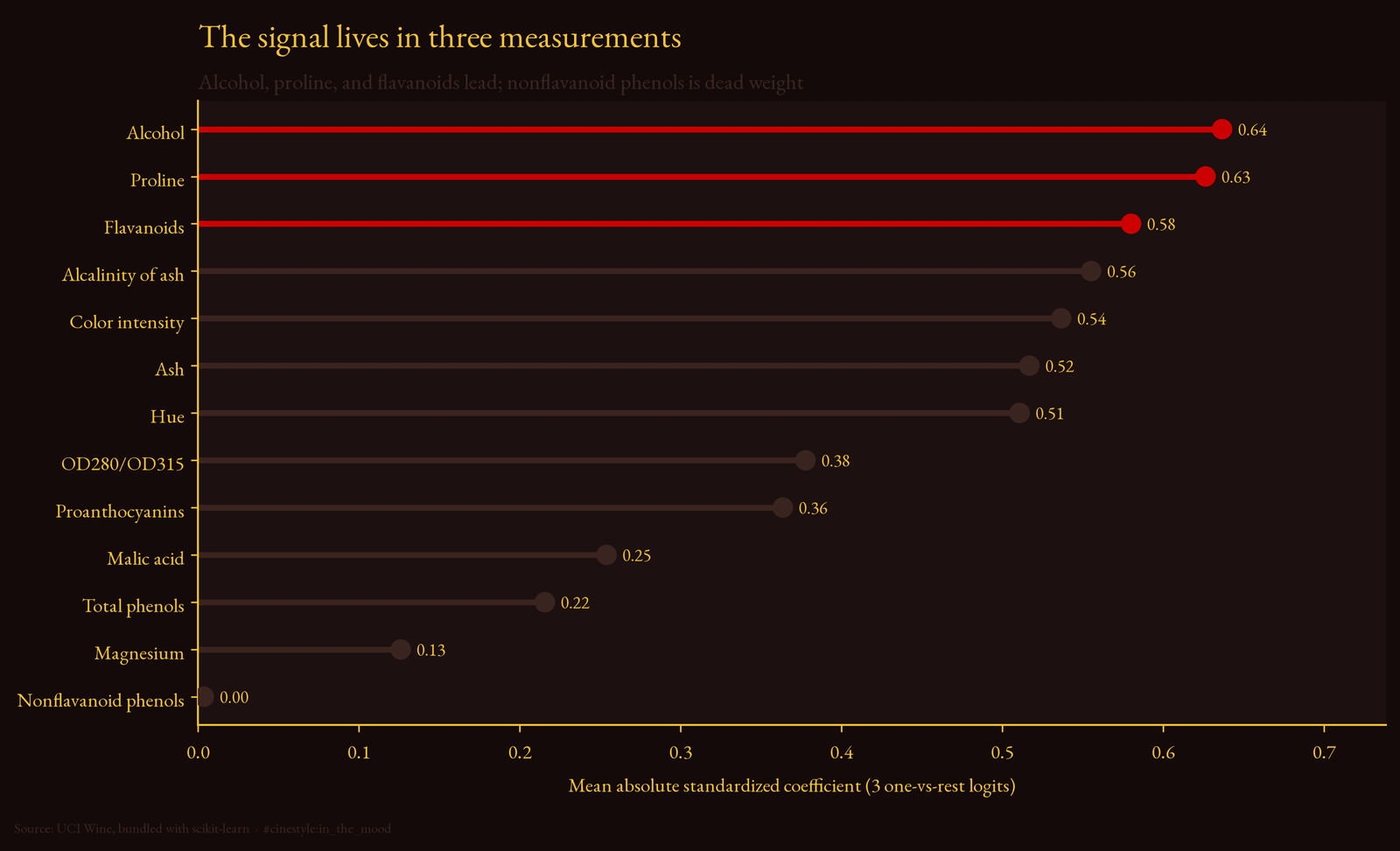
The top of the list: alcohol (0.64), proline (0.63), flavanoids (0.58). After that the coefficients sag gently. Alcalinity, color intensity, ash, and hue all cluster in the 0.51 to 0.56 band, contributing but redundant. And right at the bottom sits nonflavanoid phenols, with a mean coefficient of 0.0035, effectively zero.

I half-expected color intensity to rank higher. It is there, fifth, but the logit leans harder on alcohol and proline, which you cannot see at all. The eye trusts color; the chemistry does not.

Two features, and the honest stumble

So I cut down to the top two, alcohol and proline, and refit. 85.2%. That is the part I want to be honest about, because the clean version of this story would have two features nailing it. They do not. Eight bottles out of 54 wrong. You can see why in the decision regions.

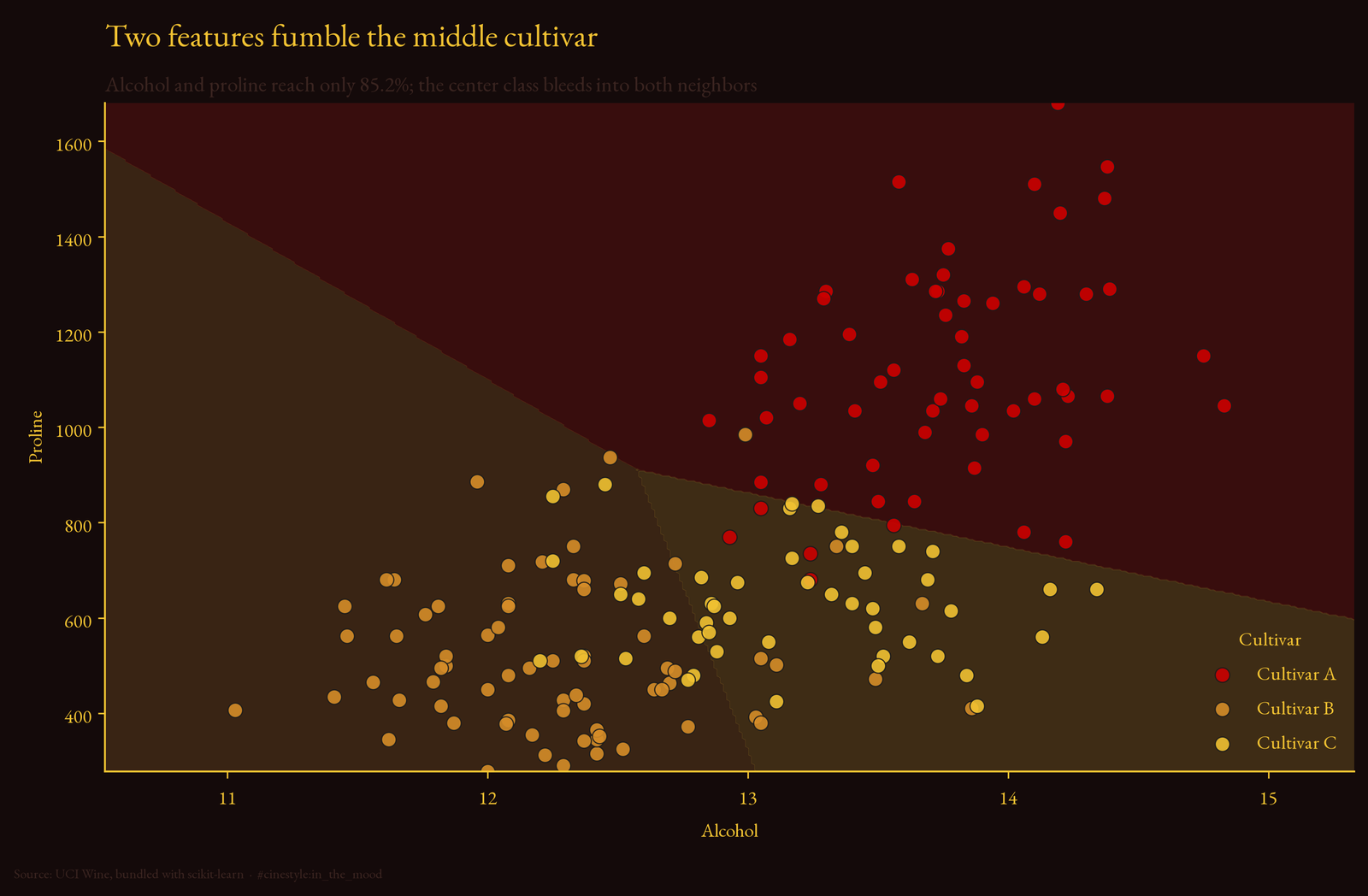
Two of the cultivars sit in tidy corners, but the third smears across the middle and bleeds into both. Alcohol and proline pull the two extremes apart and leave the middle cultivar ambiguous. Two features draw two useful boundaries and fumble the third.

Add flavanoids, the third-ranked feature, and it snaps into place: 94.4%, three bottles wrong instead of eight. Flavanoids is the axis that separates the middle group from its neighbors. That is the real finding here. Not “fewer features always work,” but: there is a specific third measurement that resolves the one ambiguity the first two leave open.

To check I was not just rediscovering my own ranking, I tried the trio a domain person might pick blind: proline, flavanoids, color intensity. That trio also scores 94.4%. When a problem is this separable, several reasonable three-feature sets land in the same place.

Where the small sample bites

Here is where I stop trusting any single number. 178 rows is small. A 54-row test set means each misclassification moves accuracy by 1.9 points, so “98.1%” and “94.4%” are both fuzzier than the decimals suggest.

So I ran 5-fold stratified cross-validation instead of leaning on one lucky split.

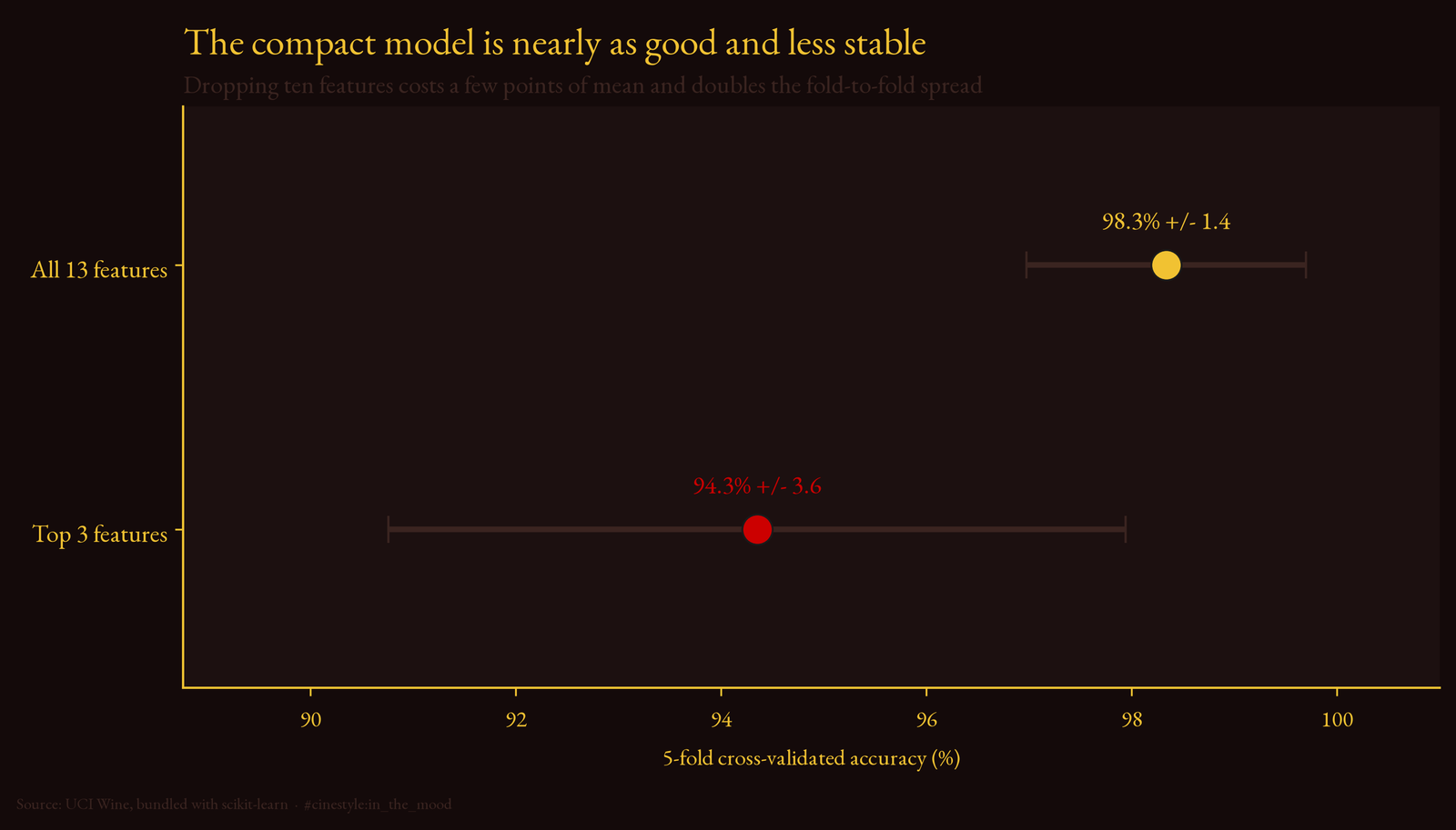
The full model: 98.3% plus or minus 1.4%. The three-feature model: 94.3% plus or minus 3.6%. Two things to read off that. First, the test-set numbers were not a fluke. The cross-validated means land right on top of them. Second, look at the spreads. The three-feature model’s standard deviation is more than double the full model’s. Dropping ten features costs you about four points of mean accuracy and, just as real, makes the result wobblier fold to fold. With this few samples, that variance is not a rounding error you get to ignore.

That is the honest tradeoff. The compact model is nearly as good on average and noticeably less stable. Whether you would ship it depends on whether four points and some fold-to-fold jitter matter more than carrying ten fewer measurements. One more wrinkle from the feature-count curve: eight features scored 100% on this test split, better than all thirteen. On a 54-row test set I read that as one lucky bottle, not a reason to prefer eight.

Why it was always going to be this easy

The PCA tells you the answer before any classifier runs. Standardize the 13 features, project to two dimensions, and the first component explains 35.7% of the variance, the second 19.2%, for 54.9% combined.

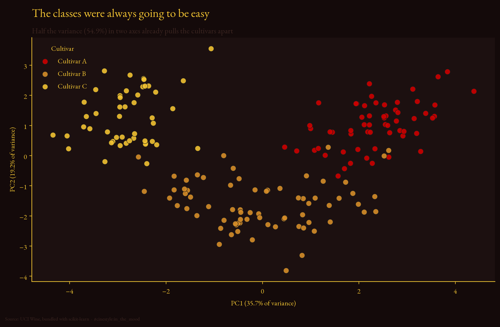
Just over half the variance in two axes, and the three cultivars fall into three visually distinct clumps with only light overlap at the seams. When your classes separate that cleanly in a linear projection that throws away 45% of the variance, a linear classifier on a handful of raw features was always going to win. There is no twisted boundary for a deep model to find.

This is a tiny, clean, almost suspiciously well-behaved dataset, and I will not pretend a Saturday with 178 rows generalizes to your production problem. But the instinct it pushes against is worth keeping. Reach for the linear model and the feature ranking first. If three columns get you to 94 and the full set gets you to 98, you have learned something real about the problem, which is more than a 98% black box ever tells you. A model that explains itself beats one that merely scores well.